
A Radar Scope on the Arduino UNO Q: Multi-Target Tracking with the Ai-Thinker RD-03D mmWave Sensor
UNO Q with a 24 GHz radar wired to the board to build a live radar scope - the MCU turns a binary sensor stream into three tracked targets, and the Linux side draws them sweeping across a web dashboard. Along the way, a proper look at how FMCW radar works, all showing the strength of mmWave radar.

Tracking with the low-cost RD-03D mmWave Sensor
This article is Part 4 of a series on the Arduino UNO Q:
- Getting to know the UNO Q: two brains, one board, and Zephyr underneath
- A real application: an AI Brick, a camera, and a presence lamp
- Under the hood: vanilla Zephyr on the UNO Q's Cortex-M33
- This guide: a live radar scope with a 24 GHz mmWave sensor
- Sensor fusion: radar meets camera (coming soon)
- The UNO Q becomes the hub of a Thread sensor fleet (coming soon)
The Bridge patterns come from Parts 1 and 2, and Part 3 turns out to matter far more than expected: its devicetree tour answers a question about the header UART that would otherwise have cost significant time.
Part 3 of this series ended with a comet sweeping the UNO Q's LED matrix, which is a pretty animation but is low on function. This part integrates the UNO Q with real-world sensing. We wire an Ai-Thinker RD-03D, a low-cost 24 GHz mmWave radar module (€7-€10), to the UNO Q's header UART, and build a live radar scope web and LED matrix display (See Video 1): the microcontroller parses the sensor's binary stream into three tracked targets, and the Linux side draws them drifting across a top-down scope in your web browser, and on the LED matrix in the bonus section. Walk across the room and watch yourself tracked, in real time, by the small UNO Q board without any external processing.
Video 1. The final outcome of this article (and the bonus LED matrix) -- the mmWave radar sensor tracking two people in the room and displaying a web interface using only the Arduino UNO Q and the RD-03D mmWave radar.
The application follows the series' format (real-time work on the MCU, presentation on the MPU, one small message crossing the seam between the MCP/MPU), but this part is unique with the sensor itself. mmWave Radar has become the most interesting thing to happen to presence sensing in a decade, and the RD-03D is an unusually capable sensor, so before any wiring we will give it the full treatment: what it actually measures, how FMCW radar works, and why you would choose it over the PIR sensors and cameras it competes with. There is an interactive demonstration to go with that section, because the signal processing behind a radar frame is one of those topics where moving sliders can help you understand some fairly complex equations.
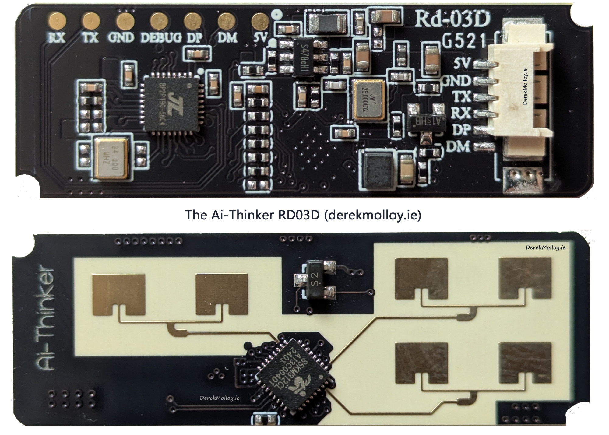
The sensor: what the RD-03D actually is
The RD-03D is a complete 24 GHz radar system on a small board: a radar transceiver chip, one transmit antenna and two receive antennas printed directly on the PCB as copper traces, and an onboard processor that does all the radar signal processing and hands you finished answers over a UART. That last point is worth underlining before the physics: you do not receive radar echoes from this module, you receive up to three simultaneously tracked targets, each with an X/Y position in millimetres and a radial speed, updated many times per second. The hard mathematics happens on the module, and a later section shows you exactly what that mathematics looks like.
Note what is not in that table. There is no "distance" field: range is something you compute from X and Y, and the article's canvas code does exactly that with Math.hypot. There is no raw data of any kind. And there is no classification: the module reports that something moved at a place, not what it was.
How FMCW radar works, in one page
The RD-03D is an FMCW (Frequency-Modulated Continuous-Wave) radar, and the concept requires attention because it explains every capability in the table above. A pulsed radar (the movie version) shouts and times the echo. That is hopeless indoors: light crosses a room in nanoseconds, so a target three metres away returns its echo about 20 ns late, and nothing in this price class is going to timestamp nanoseconds directly.
FMCW sidesteps the problem entirely. It transmits continuously, but sweeps its frequency: it emits a "chirp" that climbs smoothly through a band around 24 GHz, over and over. The reflection that comes back from your body is a copy of that chirp, delayed by the round-trip flight time. Because the transmitter has moved on in frequency during that delay, the received and transmitted signals differ in frequency at any instant, and mixing them produces a low-frequency "beat" tone whose pitch is proportional to your distance. Range measurement becomes tone measurement, and tone measurement is what small, cheap chips and Fourier transforms are extremely good at.
Two relationships carry all of it:
- τ = 2R/c, the round trip. Twenty nanoseconds at three metres.
- fb = S·τ, where S is the ramp slope in hertz per second. Multiply a nanosecond delay by a slope of megahertz-per-microsecond and the result lands somewhere an ordinary ADC can sample.
- R = cτ/2 = c·fb / 2S, which is the equation you actually came for. Substituting the first relationship into the second and rearranging gives range directly in terms of the measured tone: read the beat frequency, divide by the ramp slope to recover the delay, and halve it because the wave made the trip twice. Every quantity on the right is either a constant or something you chose when you designed the chirp, so a frequency measurement is a distance measurement. For a slope in the region of a few megahertz per microsecond, that works out at roughly ten to twenty kilohertz of beat tone per metre of range, which is why an audio-grade ADC is enough to see across a room.
Velocity comes almost free. If you are moving, each successive chirp finds you a fraction of a wavelength closer or farther, which rotates the phase of your beat tone from chirp to chirp; the rate of that rotation is your radial speed. And direction comes from the second receive antenna: an echo arriving from off-centre reaches the two antennas at minutely different path lengths, producing a phase difference between them that encodes the angle of arrival. Distance plus angle gives you the polar coordinates; the module multiplies it out and hands you X and Y. One transmit antenna, two receive antennas, and three quantities measured: range from beat frequency, speed from chirp-to-chirp phase, angle from antenna-to-antenna phase.
The 24 GHz carrier matters too, and not only because that ISM band is licence-free worldwide. Its wavelength is about 12.5 mm, and a radar's sensitivity to motion improves as its wavelength shortens: the phase change produced by a target moving a distance ΔR is Δφ = 4πΔR/λ, so the smaller λ is, the more phase you get per millimetre of movement. At 12.5 mm, a chest wall moving a few millimetres with each breath produces a large, easily measurable phase rotation. A radar that can see breathing can, in principle, hold presence on a person who has stopped moving, which is precisely the thing the previous generation of presence sensors could not do.
The picture the module hides from you
Everything above describes what happens to one chirp from one target. A real radar processes a whole frame of chirps against a whole room, and the result is a two-dimensional image called a range-Doppler map. The RD-03D computes one of these several hundred times a second and never lets you see it; what arrives on the UART is the set of calculated tracks.
I have built an interactive demonstration of that pipeline, because it is much easier to move a slider than to read an equation:
A nanosecond of delay, in megahertz
Radar has an awkward problem: light covers a room in nanoseconds. A target three metres away returns its echo 20 ns late, and no microcontroller on earth is going to timestamp that directly.
FMCW sidesteps it. Transmit a frequency ramp instead of a pulse, then compare what comes back against what is going out right now. The echo is a copy of the ramp, shifted slightly in time, which means it is also shifted in frequency, because the ramp has moved on while the echo was in flight. Mix the two and the difference is an audio-to-megahertz tone you can simply sample.
- τ = 2R/c is the round trip. Tens of nanoseconds indoors, which is why the ramp's delay is drawn exaggerated above; at true scale the two lines would sit on top of each other.
- fb = S·τ. Multiply that delay by the ramp slope and it lands in the megahertz. Range has become frequency, and frequency is what an FFT is for.
- Everything follows from the slope. Steeper ramp, more hertz per metre; the ADC's sample rate then sets how far you can see before the tone exceeds it.
Throughout this widget the chirp repetition interval is taken as equal to the ramp time. A real device inserts idle time between chirps for the synthesiser to reset, so its Tr is longer than its ramp, and both the frame time and the unambiguous velocity scale with that longer figure.
One chirp, one FFT, and every target in the beam appears as a peak at its own frequency. The resolution is not a property of the FFT. It is set entirely by how much bandwidth you swept: ΔR = c / 2B. Change the FFT length below and watch ΔR refuse to move.
Two targets at 3 m, separated by the slider. Turn the window off and the sidelobes appear: a rectangular window rings at −13.3 dB, which is loud enough to bury a small target sitting beside a large one. Hann trades about 60 % more mainlobe width for −31.5 dB sidelobes, and that trade is usually worth making.
Velocity does not come from the range peak moving. Over one frame it barely budges. It comes from phase. Each chirp measures the same target a few tens of microseconds later, and if the target has moved even a fraction of a wavelength, the phase of its peak has rotated. Stack the chirps, watch the rotation, and a second FFT reads off the speed.
Push the velocity up and watch the phase step grow. The moment it passes 180° per chirp, the measurement is finished: a rotation of 200° and a rotation of −160° are the same set of samples, and the FFT always reports the shorter way round. That single fact is the whole of Doppler ambiguity.
This is what the whole chain is for, so it is where the demo opens. The walkthrough that builds it starts at .
Both FFTs together give a 2D map: range across, velocity up. This is the frame a radar actually produces. Not points, not objects, just an image where energy sits at the range and speed of whatever put it there. Everything after this, clustering and tracking and classification, is working on this picture.
- The zero-Doppler line is the wall, the furniture, the floor. It is usually the strongest thing in the frame and it is never what you want. Tick remove zero-Doppler: subtracting each range bin's mean across chirps deletes everything stationary, in one pass, and a person breathing four metres behind a sofa suddenly stands out. That is how presence sensors work.
- Two targets at one range are separable if their speeds differ, which no camera pixel can do. Try the two people, same range preset.
- This map is a tensor. Shape (range × Doppler), one channel, real-valued. If you have fed a spectrogram to a CNN you already know what to do with it.
On the sign: this model dechirps as transmit minus receive, which is the choice that puts range at a positive beat frequency. The same arithmetic then makes a growing range a positive Doppler bin, so upward on this map is away from the radar. Half the literature draws it the other way. Neither is wrong, but a pipeline that mixes the two will track every target backwards, so it is worth checking against your own silicon before you trust an axis.
Here is the knob that breaks it. The ramp time sets how often you sample a target's phase, and that sampling has a Nyquist limit like any other: vmax = ±λ / 4Tr. Anything faster does not disappear. It reappears somewhere else on the map, wearing a completely plausible velocity.
- Only the ramp time appears in the formula. Bandwidth and sample count do not, and the sliders will show you that: drag bandwidth from 0.25 to 4 GHz and vmax does not move at all. The coupling on real hardware is indirect. Your ADC has a top sample rate and your synthesiser has a top slope, so buying more samples or more bandwidth means buying a longer ramp, and the longer ramp is what costs you the velocity. There is no setting that is good at everything, which is why a chirp configuration is a profile chosen per application rather than a default.
- Higher carrier cuts both ways. 77 GHz resolves velocity roughly three times more finely than 24 GHz, and folds at roughly a third of the speed. Switch the carrier and watch both numbers move together.
- Real systems cheat. Alternate two slightly different chirp repetition intervals and the ambiguities land in different places, so the true velocity is the one both agree on. Cheap in silicon, and it is why production chirp configurations look so untidy.
The reason this matters on the edge: the map above is not free, and it arrives hundreds of times per second whether anything asks for it or not.
- The FFT is not your bottleneck. A full range-Doppler frame is about half a million flops. A single 3×3 convolution into 16 channels, over that same map, is four times as much again, and that is one layer. If a radar pipeline is missing its deadline, look at the model, not the transform.
- The ADC is the real pressure. Raw samples arrive at tens of megabytes per second and nothing downstream wants them. The FFT is best understood as a compression stage that happens to be physically meaningful, which is exactly why it belongs on the sensor rather than on the host.
- Frames are cheap, decisions are not. At 300 frames per second you can afford to average, or to run a model on every tenth frame and track in between. Choosing what not to compute is most of edge design.
Figures are computed from the settings you chose on the previous tabs. The headline flop count is the two transform stages only. Windowing, magnitude, memory stalls and CFAR are all excluded, though magnitude is costed separately in the table so you can see how little it adds. Treat these as a floor rather than an estimate.
That demonstration is the reference for every radar post on this blog, and it covers the full chain properly. What follows here is the part of it that bears directly on the module in front of you, so feel free to skim ahead to the wiring.
The demonstration walks the chain in six steps, and everything in it is computed live in the browser. Four of those steps say something specific about the sensor sitting on your bench:
- Range resolution is bandwidth, and nothing else. The demo's one chirp → range tab puts two targets close together and lets you slide them apart. The rule is ΔR = c / 2B, and notice that the carrier frequency does not appear in it at all: only the width of the sweep matters. Drag that tab's bandwidth slider down to its 0.25 GHz minimum, which is what the 24 GHz ISM allocation permits, and the resolution readout settles at about 60 cm. That is the finest range resolution physically available to the RD-03D. Slide the two targets closer than that and they merge into a single peak, with a warning telling you that no FFT length, interpolation or averaging will recover them. Two people standing within 60 cm of each other at the same angle are one target, permanently. This is also why 60 GHz parts exist: they get several gigahertz of bandwidth and resolve to a few centimetres.
- Velocity comes from phase across chirps, not from the peak moving. The third tab plots the phase of a target's range peak chirp by chirp and runs the second FFT over it. Over one frame the target barely moves in range; the entire velocity measurement lives in a rotation of a few degrees per chirp.
- The zero-Doppler line is where static presence is determined. On the map tab, the strongest thing in the frame is almost always the horizontal stripe at zero velocity: the walls, the floor, the furniture. Tick remove zero-Doppler and the demo subtracts each range bin's mean across the chirps, deleting everything stationary in a single pass. This is MTI (moving target indication), and it is the mechanism the warning above is about. A design that runs aggressive clutter cancellation gets clean, stable tracks on walking people and loses the breathing person entirely; a design tuned for presence keeps the near-zero-Doppler bins and accepts more false alarms. The RD-03D has made that choice for you, in firmware.
- Aliasing is real but is not your problem here. The fifth tab is the one that breaks things: sample a target's phase once per chirp and you inherit a Nyquist limit like any other sampled system, vmax = ±λ / 4Tr. Past that, a fast target does not vanish, it reappears at a plausible but wrong velocity. It is worth understanding because it is the typical radar failure that no downstream tracker can detect. It is also worth knowing that at 24 GHz the long wavelength makes the limit generous, tens of metres per second for typical ramp times, so pedestrians do not fold. Switch the demo's carrier to 77 GHz and watch the same target start lying to you, and you have the reason automotive radar configurations look so untidy.
Which sets up an interesting counterfactual for this series. Buy a radar that exposes its raw data cube instead (the Texas Instruments IWR-class parts, or a 60 GHz module with an SPI data path) and that range-Doppler transform becomes a heavy workload, at fast data rates, that has to land somewhere. On the UNO Q it would land on the A53s and their NEON units, with the MCU reduced to timing and control. Same board, opposite division of labour, and the choice is made entirely by where the sensor vendor decided. Part 5's fusion work is where that question gets interesting.
Why mmWave is such a good sensor type
Every presence-sensing technology is a bundle of trade-offs, and mmWave's bundle is surprisingly strong. Against the alternatives:
Three rows deserve expansion:
- Still-person detection is the practical revolution of the sensor class. Everyone has sat in a suddenly dark room where the PIR-driven lights decided there is nobody present. PIR detects change in infrared; a settled occupant produces none. A mmWave sensor holds a lock on a breathing, fidgeting, and other micro movement, which is why the technology has taken over the serious end of occupancy sensing. (The smart-home products in this class do the same job, though not always at the same frequency: Aqara's FP2, for instance, is a 60 GHz part rather than a 24 GHz one.) The RD-03D does it, which I did not take for granted and tested; the "Running it" section has the result.
- Mounting through materials changes product design. A 24 GHz wave passes through plastic, wood, and plasterboard with modest loss, so the sensor needs no window, no lens, no visible presence at all: it can sit inside an enclosure, behind a bookshelf panel, above a ceiling tile. Every other technology in the table above must see or hear the room directly.
- Privacy is the argument that decides real deployments. Part 2's camera can classify what it sees, but it sees: pointing one at a bed or a bathroom is socially unacceptable and even legally fraught, however locally the inference runs. The radar's output is the numbers; there is no image to leak, which makes it deployable in exactly the rooms where presence sensing is most useful. The counterpoint is the new row in that table: the camera knows a person from a dog, and the mmWave radar does not. Part 5 of this series fuses the two so each covers the other's blind spot.
The RD-03D's specific capability within the mmWave family is the multi-target tracking with coordinates. Simpler modules in the same price class (the LD2410, Ai-Thinker's own RD-03 and RD-03E) output presence flags and a distance. This one runs a tracking algorithm on the module and maintains identity and trajectory for up to three targets, which is what turns "the room is occupied" into "two people, one at the sofa, one walking toward the door at 0.8 m/s", and is what makes a radar scope application here possible at all.
Wiring, and the UART you are actually borrowing
Four wires connect the module: 5 V, GND, and the UART pair. On the UNO Q, the R3 header's serial pins are the home, and here Part 3's devicetree is useful, because the obvious guess about those pins is wrong. The obvious guess, given this board's architecture, is that D0 and D1 run inward to the Qualcomm MPU the way a classic UNO's D0/D1 run to its USB-serial bridge chip. They do not. Part 3 established the actual arrangement by reading arduino_r3_connector.dtsi and arduino_uno_q-common.dtsi, and it is the opposite:
usart1(PB6/PB7) isD1/D0, and it is what the devicetree nameszephyr,console. It goes to the header pins and nowhere else.lpuart1(PG5-PG8) is the flow-controlled internal link to the QRB2210, appearing on the Linux side as/dev/ttyHS1witharduino-routerholding it open. That is the Bridge.
So the header serial is not shared with Linux, and there is no contention with the MPU to worry about. What there is contention with is the MCU's own console, which is a smaller problem but a real one: the Zephyr-based Arduino core has CONFIG_UART_CONSOLE=y compiled in from the board's defconfig, and anything it prints at 115200 lands on the same two pins your radar is talking to at 256000.
/dev node for it, no way for a Python script to open it, no clever workaround. Part 3's closing observation was that on the UNO Q the Linux half owns the physical resources and anything you want, you take from it; this is the one case that runs the other way. The microcontroller owns this sensor outright, which decides the architecture.The table below shows the wiring configuration for the RD-03D. The colours are the values I chose, as in the images and videos that follow:
Getting from the module to the header: the connector
Four wires sounds like a five-minute job, and it is, but only once you have solved a small mechanical problem – The RD-03D does not have pins. It has a socket, and that socket is not a breadboard pitch. The module terminates in a 4-way, 1.25 mm pitch connector, usually written on parts listings as 1×4P 1.25 mm. That description is where the trouble starts, because two different connector families share that pitch and the listings rarely say which one they mean. The RD-03D takes the Molex PicoBlade-compatible part, sold as PB1.25, and not the JST GH part that looks identical in a photograph. The one on my module mated with a PB1.25 housing, which is the only test that settles it. The important number is the pitch: 1.25 mm is less than half the 2.54 mm of a breadboard, of a DuPont jumper, and of the UNO Q's own R3 headers.
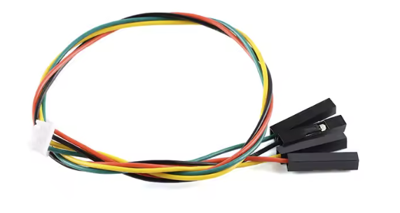
So you need a pigtail, as illustrated in Figure 3, and you have four routes to one:
- Use the cable that came in the bag. Many RD-03D listings include a matching 4-way pigtail: a keyed 1.25 mm plug at one end, and bare, tinned, or DuPont-terminated flying leads at the other. This is the intended path. Order a spare with the module, because the housings are small and easy to damage.
- Buy a ready-made adapter. Search for a "1.25 mm 4P to 2.54 mm DuPont" cable. Since the UNO Q's headers are 2.54 mm female, you want male DuPont pins on the board end, but they are hard to come by.
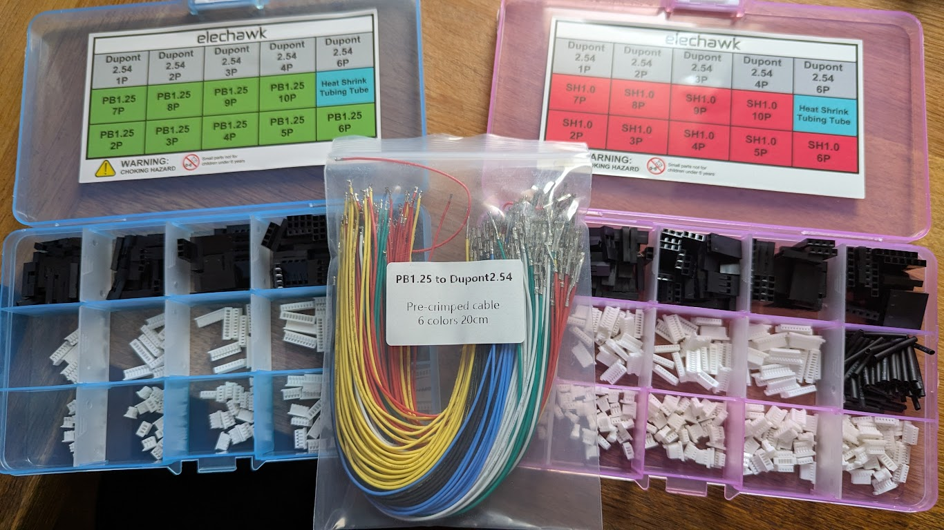
- Buy a pre-crimped assortment kit. This is what I do now, and it has retired the problem permanently. Kits such as Elechawk's ship a few hundred 20 cm wires with a terminal already crimped on each end, plus boxes of empty housings in every pin count. You assemble whatever cable you need by pushing the terminals into a shell with the supplied tweezers, so there is no crimp tool, no ruined terminals, and no time lost to being one cable short. They cost little and the box outlasts several projects.
- Crimp your own, if you already own a 1.25 mm crimp tool and a bag of housings. Worth it if you expect to build several; entirely not worth it for one.
Two more practical notes. Some RD-03D boards expose plated through-holes or castellated pads alongside the connector; if yours does and the installation is permanent, soldering directly to those is far more robust than relying on the socket. And whichever route you take, give the cable strain relief. A strip of tape or a blob of hot glue securing the cable to whatever the module is mounted on costs nothing and saves that hour, particularly on robotic and other moving platforms.
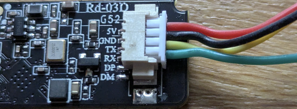
Its UART lines, however, are 3.3 V: the UNO Q's headers are 3.3 V logic too, so D0 and D1 connect straight across with no level shifter. Do not let the 5 V on the supply pin tempt you into thinking the data pins are 5 V as well, and do not assume a module labelled for 5 V is 5 V-tolerant on its inputs.
Two consequences for this build. Take VCC from the UNO Q's 5V header pin, which is fed from the board's USB-C supply and has the headroom the 3V3 rail does not. And treat a brownout as a possible issue when debugging: a module resetting mid-frame under transmit current presents as intermittent parse failures, which is a difficult thing to chase from the software side. If you are powering the board from a weak charger rather than a proper 5 V/3 A supply, check that first.
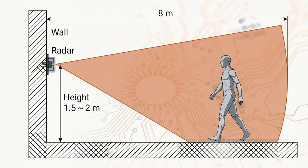
Mount the module standing on its edge, antennas facing the room, at roughly chest height if you can (as per Figure 2): the X axis then runs across the sensor's face, Y points outward into the room, and the ±60° field of view lies in that horizontal plane. Which way up it stands turns out to matter more than you would expect, so there is a photograph and an explanation in Running it before you switch anything on.
The protocol, and who should parse it
The RD-03D speaks a compact binary protocol, and parsing it is a nice exercise in exactly the kind of work a microcontroller should own. Two frame families matter.
Command frames (you → radar) are bracketed by FD FC FB FA ... 04 03 02 01. The one command we need selects multi-target mode (the byte at position six is 0x90 for multi, 0x80 for single):
FD FC FB FA 02 00 90 00 04 03 02 01 -> "track up to three targets"
Report frames (radar → you) arrive continuously, roughly every hundred milliseconds: a 4-byte header AA FF 03 00, then three 8-byte target slots (an absent target is eight zero bytes), then the tail 55 CC. Thirty bytes per report. Each slot:
That last field is a per-target resolution figure rather than the target's distance, and the previous section explains where it comes from: with 250 MHz of sweep, expect something in the region of 600 mm. Range itself is not transmitted at all; you compute it from X and Y.
The sign-flag encoding is the protocol's one usual point: rather than two's complement, the top bit is a sign flag (set = positive, clear = negative) and the low fifteen bits are the magnitude. Miss this and every leftward target teleports to the far right of your scope. In code:
static int16_t rd03d_decode(uint16_t raw)
{
    /* Sign bit SET means positive: strip it and the magnitude remains.
     * Sign bit CLEAR means negative, and the cast is safe precisely
     * because that bit is clear, so raw <= 0x7FFF and -(int16_t)raw
     * cannot overflow.
     */
    return (raw & 0x8000) ? (int16_t)(raw & 0x7FFF) : -(int16_t)raw;
}
So why does this belong on the microcontroller?
It is tempting to reach for the argument the baud rate suggests: 256,000 baud sounds like a data rate that only a real-time processor could survive. However, thirty bytes ten times a second is 300 bytes per second. A Python script could read that in its sleep; so could a Raspberry Pi, a laptop, or a wristwatch. Average throughput is not the argument. What is true, is a burst constraint and an ownership fact:
- The burst is real even though the average is not. Thirty bytes at 256,000 baud take about 1.17 ms, delivered as a continuous run of characters roughly every 100 ms. During that burst, bytes arrive every 39 µs. The STM32U585's USART has an 8-byte receive FIFO, so during those 1.17 ms the reader has roughly 312 µs of slack before it drops characters. That is a perfectly ordinary microcontroller requirement and an awkward one for a general-purpose OS, but notice how narrow the claim is: it applies for one millisecond in every hundred.
- The pins are the actual argument. As the wiring section established, the header UART is wired to the STM32 and to nothing else. There is no design in which Linux parses this stream, because Linux cannot reach it. Everything else follows from that.
Now count what crosses the seam between the MCU and CPU. Into the MCU: a burst of binary frames on a hardware UART, demanding a byte-level state machine that tolerates torn frames and garbage. Out of the MCU: at most nine small numbers, ten times a second. The MCU is not only relaying; it is converting a wire format into an application fact, next to the pins that carry it, which is why the Python side of this project will be quite short. That is the same "what is the smallest thing that can cross the boundary?" question from Part 2, answered again.
The App
Create a new App in Arduino App Lab, call it radar_scope, and add the Web UI Brick from the Bricks panel (it is listed as Web UI - HTML). There is no AI Brick this time, because the intelligence is already on the sensor.
App Lab does the scaffolding for you. Creating the App gives you the folder skeleton with a sketch/ directory containing both sketch.ino and its sketch.yaml build manifest, and adding the Brick writes the app.yaml entry and creates the assets/ folder the Web UI serves from. You do not have to hand-write any of that.
Adding the Brick also populates assets/ with the client-side plumbing, including libs/socket.io.min.js. That matters more than it sounds, because socket.io is how the page and your Python talk to each other, and it is already sitting there.
What App Lab gives you is a scaffold, not a finished App, and the one thing it cannot guess is the page itself. The Web UI Brick's assets/index.html starts as an empty stub containing <!-- Add your HTML here -->, and the canvas scope later in this article is what replaces it. If you were expecting a dashboard to appear ready-made, that is not what the Brick does: it serves whatever you put in assets/, and to begin with there is nothing to serve.
Here is the app.yaml App Lab writes once the Brick is added. You do not type this, but it is worth reading, because it is short enough to understand completely and it is the whole declaration of what this App needs:
name: radar_scope
description: ""
ports: []
bricks:
- arduino:web_ui: {}
icon: 😀
Four of those five lines repay a moment's attention, because the shape of this file is the shape of every UNO Q App:
descriptionandiconare defaults, empty and a smiley respectively. App Lab does not ask you for either, which leads directly to the box below.ports: []is empty, and correctly so. This list opens network ports for things outside the board to reach. Part 2's App needed8080there so a phone could stream camera frames in; nothing here comes from off-board, because our sensor arrives on a UART. The web page itself is served on port 7000 by the Brick, which is the Brick's business rather than yours, so it does not appear.arduino:web_ui: {}is a Brick with no options. Those empty braces are where per-Brick configuration goes when a Brick needs any: Part 2's vision Brick carried adevices:list in exactly that position to bind it to a remote camera. Ours needs nothing, so the map is empty.
app.yaml but will not let you edit it. This surprises everyone, because the editor displays the file exactly like any other and then refuses keystrokes. Nothing in this project needs the manifest changed, so you can read past it, but the moment you want a different description or icon, or a Brick option the panel does not expose, you have to go around App Lab: ssh arduino@.local and then nano ~/ArduinoApps/radar_scope/app.yaml. Then press Run in App Lab, or arduino-app-cli app start ~/ArduinoApps/radar_scope, so the changed manifest is picked up.Which leaves this folder shape, where everything unmarked is created for you:
radar_scope/
├── app.yaml                    <- App Lab, when you add the Brick
├── assets/
│   ├── index.html              <- YOURS: replaces the empty stub
│   └── libs/
│       └── socket.io.min.js    <- App Lab, with the Brick
├── python/
│   └── main.py                 <- YOURS
└── sketch/
    ├── sketch.ino              <- YOURS
    └── sketch.yaml             <- App Lab
Three files to write, then: the sketch, the Python, and the web page. They are the next three sections.
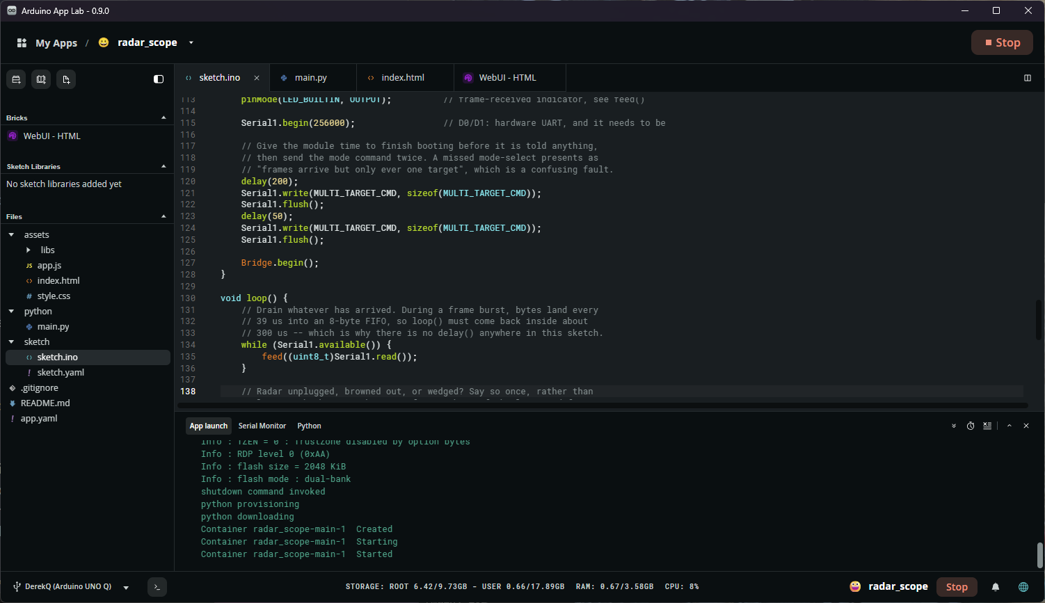
radar_scope App in App Lab, with the Web UI Brick added and the generated folder structure in the sidebar. Everything visible here was created by App Lab; only index.html, main.py and sketch.ino are ours to write.Design before code: which way does the data flow?
Parts 1 and 2 both pushed data in the same direction. Linux measured something (CPU load, then a person's presence) and called a function the sketch had provided. The MCU was always the callee. This project reverses it, and that is new ground for the series. The radar produces data on its own schedule; nobody on the Linux side knows when a frame has arrived. There are two ways to handle that, and the choice has consequences well beyond style:
- Poll: Python asks the MCU for the current picture ten times a second, and the sketch returns it. This keeps the familiar MPU-calls-MCU direction, but it needs Bridge return values, which nothing in this series has exercised. It also introduces two problems. Polling at 10 Hz for data produced at 10 Hz means aliasing, so you will silently duplicate some frames and drop others. And because the sketch's returned picture is read by the RPC handler while
loop()may be part-way through rewriting it, you inherit a shared-state race between two thread contexts. - Push: the sketch calls a function Python has provided, the moment a frame is parsed. No aliasing, no polling latency, no shared state at all, because the data never has to sit anywhere waiting to be collected.
Push is clearly correct here, and it deletes an entire class of bug rather than managing it. The one thing it needs is a Bridge capability the series has not used before: a call travelling from the microcontroller to Linux, against a function that Python provided. That works, and the rest of this article is built on it.
The sketch (sketch/sketch.ino)
// radar_scope -- MCU half.
// Owns the RD-03D: selects multi-target mode, then runs a byte-level state
// machine over the report stream. Each complete frame is parsed and pushed
// straight across the Bridge, rate-limited. Nothing is stored between
// calls, so there is no shared state for an RPC thread to race against.

#include "Arduino_RouterBridge.h"

#define MAX_TARGETS   3
#define FRAME_LEN     30            // AA FF 03 00 + 3*8 bytes + 55 CC
#define PUSH_MS       100           // don't flood the Bridge with frames
#define STALE_MS      500           // silence for this long => radar is gone

static const uint8_t MULTI_TARGET_CMD[] = {
    0xFD, 0xFC, 0xFB, 0xFA, 0x02, 0x00, 0x90, 0x00,
    0x04, 0x03, 0x02, 0x01
};

static const uint8_t HDR[4] = { 0xAA, 0xFF, 0x03, 0x00 };

static uint8_t  frame[FRAME_LEN];
static uint8_t  pos = 0;
static uint32_t last_frame_ms = 0;   // last good frame from the radar
static uint32_t last_push_ms  = 0;   // last message we sent to Linux
static bool     reported_gone = true;

// The protocol's sign-flag encoding: top bit SET means positive, CLEAR
// means negative; the low 15 bits are the magnitude. NOT two's complement,
// and this is the classic RD-03D parsing mistake. The cast in the negative
// branch is safe precisely because the top bit is clear there.
static int16_t rd03d_decode(uint16_t raw)
{
    return (raw & 0x8000) ? (int16_t)(raw & 0x7FFF) : -(int16_t)raw;
}

// Build "x,y,v;x,y,v;x,y,v" with an empty field for an absent slot, so the
// SLOT INDEX SURVIVES the trip. The module tracks identity across frames;
// throwing that away here would make the browser's trails jump between
// targets whenever one of them drops out.
static String format_targets(void)
{
    String out;

    for (int t = 0; t < MAX_TARGETS; t++) {
        const uint8_t *p = &frame[4 + t * 8];

        bool present = false;
        for (int i = 0; i < 8; i++) {
            if (p[i]) { present = true; break; }
        }

        if (present) {
            int16_t x = rd03d_decode((uint16_t)(p[0] | (p[1] << 8)));
            int16_t y = rd03d_decode((uint16_t)(p[2] | (p[3] << 8)));
            int16_t v = rd03d_decode((uint16_t)(p[4] | (p[5] << 8)));
            out += String(x) + "," + String(y) + "," + String(v);
        }
        if (t < MAX_TARGETS - 1) {
            out += ";";
        }
    }
    return out;
}

// Feed one byte to the frame state machine. Resynchronises on the
// AA FF 03 00 header and validates the 55 CC tail before accepting.
static void feed(uint8_t b)
{
    if (pos < 4) {
        if (b == HDR[pos]) {
            frame[pos++] = b;
        } else {
            // Restart the hunt. A mismatched byte may itself be a fresh
            // header start, so check it before discarding.
            pos = 0;
            if (b == HDR[0]) {
                frame[pos++] = b;
            }
        }
        return;
    }

    frame[pos++] = b;
    if (pos < FRAME_LEN) {
        return;
    }
    pos = 0;                               // accept or discard, either way rehunt

    if (frame[FRAME_LEN - 2] != 0x55 || frame[FRAME_LEN - 1] != 0xCC) {
        return;                            // torn frame: drop it silently
    }

    uint32_t now = millis();
    last_frame_ms = now;

    // Toggle the built-in LED on every valid frame. This is the only
    // observability the MCU has in this project, because the radar has
    // taken the one UART that could otherwise have carried a console. A
    // flickering LED means bytes are arriving AND passing the tail check,
    // which cleanly separates "the sensor is silent" from "the sensor is
    // fine and the fault is further down the chain". One GPIO write per
    // frame is nothing; leave it in permanently.
    digitalWrite(LED_BUILTIN, !digitalRead(LED_BUILTIN));

    if (now - last_push_ms >= PUSH_MS) {
        last_push_ms  = now;
        reported_gone = false;
        Bridge.call("radar_targets", format_targets());
    }
}

void setup() {
    pinMode(LED_BUILTIN, OUTPUT);          // frame-received indicator, see feed()

    Serial1.begin(256000);                 // D0/D1: hardware UART, and it needs to be

    // Give the module time to finish booting before it is told anything,
    // then send the mode command twice. A missed mode-select presents as
    // "frames arrive but only ever one target", which is a confusing fault.
    delay(200);
    Serial1.write(MULTI_TARGET_CMD, sizeof(MULTI_TARGET_CMD));
    Serial1.flush();
    delay(50);
    Serial1.write(MULTI_TARGET_CMD, sizeof(MULTI_TARGET_CMD));
    Serial1.flush();

    Bridge.begin();
}

void loop() {
    // Drain whatever has arrived. During a frame burst, bytes land every
    // 39 us into an 8-byte FIFO, so loop() must come back inside about
    // 300 us -- which is why there is no delay() anywhere in this sketch.
    while (Serial1.available()) {
        feed((uint8_t)Serial1.read());
    }

    // Radar unplugged, browned out, or wedged? Say so once, rather than
    // leaving the browser showing a frozen ghost of the last good frame.
    uint32_t now = millis();
    if (!reported_gone && (now - last_frame_ms) > STALE_MS) {
        reported_gone = true;
        Bridge.call("radar_targets", String(";;"));
    }
}
There are a few details are worth pausing on:
- The state machine never trusts the stream. Power the radar up mid-frame, brush a jumper, or drop a byte, and
feed()falls back to hunting for the next header; the tail check discards frames that lost bytes in the middle. Serial protocol parsers that assume alignment work on the bench and fail at the demo. There is a small subtlety in the resynchronisation: when a header byte mismatches, the code checks whether the offending byte is itself0xAAbefore discarding it, which is what letsAA AA FF 03 00synchronise correctly. That naive one-byte rewind is sufficient here only becauseAA FF 03 00has no self-overlap beyond its first byte; a header that could partially match itself would need a proper KMP-style failure table. Worth knowing which situation you are in before reusing this. - The staleness path is not optional. Part 2 made this mistake into a troubleshooting entry ("the lamp reacts but never releases") and the same trap is here in a nastier form: without the
STALE_MScheck, unplugging the radar leaves the last good frame on screen forever, and a frozen blip looks exactly like a stationary person. Reporting absence is a separate job from reporting presence, and it needs its own code. - The LED is not decoration. Wiring the radar to D0/D1 costs you the MCU's console, which means that for the rest of this project the microcontroller has no way to tell you anything. One GPIO toggle per valid frame restores the single most useful fact you could want from it: is the sensor talking, and is what it sends surviving the parser? When something later goes wrong, and it will, that flicker instantly splits the problem in half. Debug output does not have to be text, and on a board that has run out of ways to speak, a blinking LED is a serial port with one bit!
- There is no shared mutable state. Compare this with the sketches in parts 1 and 2, both of which needed a
volatilevariable to hand data between an RPC handler andloop(). Hereframe[]andposare touched only fromloop()'s call chain, so there is nothing to protect. That is a direct consequence of choosing push over poll.
static volatile snapshot array, have parse_frame() write it, and provide String get_targets() for Python to call. Two things then become your responsibility rather than the architecture's. First, the snapshot is read from the Bridge's thread while loop() writes it, so write into a back buffer and publish it by flipping a single index (an aligned volatile uint8_t write is atomic on Cortex-M33; a nine-field struct copy is not). Second, add the staleness check to the getter as well as to loop(), because a poll that arrives after the radar died must return ";;" rather than a stale picture. You would also need to confirm that a sketch-provided function can return a value across the Bridge at all, and that an Arduino String survives the trip rather than needing a const char* into a static buffer. Neither is exercised by the push design, which is one more reason to prefer it.The Linux half (python/main.py)
# radar_scope -- MPU half.
# Receives target pictures pushed from the MCU, reshapes them as JSON, and
# forwards them to the browser scope. Short on purpose: the MCU already did
# the hard part, and nothing here has to be timely.

import time

from arduino.app_utils import *                    # App, Bridge (see part 1)
from arduino.app_bricks.web_ui import WebUI

ui = WebUI()

MAX_TARGETS = 3


def parse(s):
    """ "x,y,v;;x,y,v" -> target dicts, with the SLOT INDEX preserved.

    Slot identity is the module's tracking output and the browser needs it
    to keep each target's colour and trail attached to the right person.
    """
    out = []
    for slot, chunk in enumerate(s.split(";")[:MAX_TARGETS]):
        chunk = chunk.strip()
        if not chunk:
            continue
        try:
            x, y, v = (int(n) for n in chunk.split(","))
        except ValueError:
            continue                              # torn field: skip this slot
        out.append({"slot": slot, "x": x, "y": y, "v": v})
    return out


def on_targets(raw):
    """Called from the sketch, once per radar frame."""
    ui.send_message("targets", {
        "targets": parse(raw or ""),
        "ts": time.time(),
    })


# Send the page a starting state as soon as a browser connects, so a scope
# opened during a quiet moment is empty rather than blank.
ui.on_connect(lambda sid: ui.send_message("targets", {"targets": [], "ts": time.time()}))

Bridge.provide("radar_targets", on_targets)


def loop():
    # Nothing to do here: the work is entirely event-driven. The loop exists
    # because App.run() expects one, and because it is the natural place to
    # add logging or a recording tap later.
    time.sleep(1.0)


App.run(user_loop=loop)
The WebUI usage here follows Part 2's bundled example exactly: an instance, ui.send_message(event, data) to push, ui.on_connect(...) for the arrival of a browser. The transport underneath is socket.io, which is why the page below loads socket.io.min.js rather than opening a raw WebSocket.
The scope itself (assets/index.html)
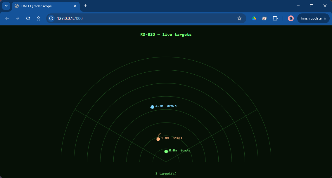
The Web UI Brick serves whatever lives in assets/; this page draws a classic top-down scope on a canvas: range rings every metre, the ±60° field-of-view wedge, and a colour-coded blip per target slot with a fading trail. The drawing is standard canvas work, and the only App-Lab-specific lines are the two socket.io calls. Four decisions in this code are worth flagging, because each one fixes a bug that the obvious version of this page has:
- Trails are indexed by radar slot, not by array position. If you iterate the received array and use its index, then the moment slot 0 disappears the slot-1 target inherits slot 0's colour and trail history, and the scope draws a line across the room between two different people. The whole point of this module is that it maintains identity; the code has to respect that.
- The scale is constrained by width as well as height. A scale derived only from the canvas height puts the ±60° wedge edges outside the canvas at full range, so the field of view silently gets clipped. Taking the smaller of the two constraints fixes it.
- The fade is redrawn, not accumulated. The tempting trick is to paint a translucent rectangle each frame and let old pixels decay. That ties the fade rate to the frame rate, which is not the data rate, so the trail length changes if the browser throttles the tab. Clearing fully and drawing each trail as an explicit alpha ramp is deterministic.
- The render loop runs on its own clock. Drawing only on message arrival means a dead radar freezes the display.
requestAnimationFrameplus a staleness check makes absence visible.
Here is the source code for assets/index.html (it is also attached at the end of this article):
<!doctype html>
<meta charset="utf-8">
<title>UNO Q radar scope</title>
<style>
body { margin: 0; background: #061006; display: grid; place-items: center;
min-height: 100vh; font-family: monospace; color: #7dff7d; }
canvas { max-width: 95vw; }
#status { font-size: 12px; opacity: 0.7; height: 1.2em; }
</style>
<h3>RD-03D — live targets</h3>
<canvas id="scope" width="720" height="420"></canvas>
<div id="status"></div>
<script src="libs/socket.io.min.js"></script>
<script>
const cv = document.getElementById("scope"), g = cv.getContext("2d");
const statusEl = document.getElementById("status");
const RANGE_MM = 8000; // scope shows the module's full 8 m
const FOV_DEG = 60;
const MAX_SLOTS = 3;
const TRAIL_MAX = 40; // ~4 s of history at a 10 Hz feed
const STALE_MS = 800; // no data for this long => go dark
const ORIGIN = { x: cv.width / 2, y: cv.height - 20 };
// Fit BOTH the range rings (height) and the widest point of the
// field-of-view wedge (width), or the wedge runs off the canvas.
const HALF_W_MM = RANGE_MM * Math.sin(FOV_DEG * Math.PI / 180);
const SCALE = Math.min((cv.height - 60) / RANGE_MM,
(cv.width / 2 - 30) / HALF_W_MM);
const COLOURS = ["#7dff7d", "#7dd4ff", "#ffb37d"];
const trails = [[], [], []]; // indexed by RADAR SLOT, not by
// position in the received array
let latest = [];
let lastMsg = 0;
function drawGrid() {
g.fillStyle = "#061006";
g.fillRect(0, 0, cv.width, cv.height);
g.strokeStyle = "#1e4d1e";
g.lineWidth = 1;
for (let m = 1; m * 1000 <= RANGE_MM; m++) { // range rings, 1 m apart
g.beginPath();
g.arc(ORIGIN.x, ORIGIN.y, m * 1000 * SCALE, Math.PI, 2 * Math.PI);
g.stroke();
}
for (const a of [-FOV_DEG, FOV_DEG]) { // field-of-view edges
const r = a * Math.PI / 180;
g.beginPath();
g.moveTo(ORIGIN.x, ORIGIN.y);
g.lineTo(ORIGIN.x + Math.sin(r) * RANGE_MM * SCALE,
ORIGIN.y - Math.cos(r) * RANGE_MM * SCALE);
g.stroke();
}
}
function drawTarget(t) {
const slot = t.slot;
const px = ORIGIN.x + t.x * SCALE;
const py = ORIGIN.y - t.y * SCALE;
const colour = COLOURS[slot % COLOURS.length];
const trail = trails[slot];
const head = trail[trail.length - 1];
if (!head || head.px !== px || head.py !== py) {
trail.push({ px, py });
if (trail.length > TRAIL_MAX) trail.shift();
}
// Explicit alpha ramp: the tail's age is measured in samples, not in
// however many times the browser happened to repaint.
g.strokeStyle = colour;
g.lineWidth = 2;
for (let k = 1; k < trail.length; k++) {
g.globalAlpha = k / trail.length * 0.8;
g.beginPath();
g.moveTo(trail[k - 1].px, trail[k - 1].py);
g.lineTo(trail[k].px, trail[k].py);
g.stroke();
}
g.globalAlpha = 1;
g.fillStyle = colour;
g.beginPath();
g.arc(px, py, 6, 0, 2 * Math.PI);
g.fill();
g.font = "12px monospace";
g.fillText(`${(Math.hypot(t.x, t.y) / 1000).toFixed(1)}m ${t.v}cm/s`,
px + 10, py);
}
function render() {
requestAnimationFrame(render);
const stale = !lastMsg || (performance.now() - lastMsg) > STALE_MS;
if (stale) {
latest = [];
for (const t of trails) t.length = 0;
}
// A slot that has gone quiet must lose its trail, or a target that
// reappears elsewhere draws a line from wherever it used to be.
const live = new Set(latest.map(t => t.slot));
for (let s = 0; s < MAX_SLOTS; s++) {
if (!live.has(s)) trails[s].length = 0;
}
drawGrid();
for (const t of latest) drawTarget(t);
statusEl.textContent = stale ? "no data from the radar"
: `${latest.length} target(s)`;
}
// Start drawing straight away, and keep drawing. The scope deliberately
// does not wait for the socket: if data never arrives we want an empty
// scope that says so, not a blank page with nothing to debug from.
render();
// The App-Lab-specific part: socket.io, and the event name main.py sends.
// Everything above is ordinary canvas work. The try/catch means a missing
// socket.io library reports itself on the page rather than silently
// stopping the script.
try {
const sock = io();
sock.on("targets", (msg) => {
// The Brick delivers the dict you handed to ui.send_message()
// verbatim, so msg IS the payload and msg.targets is the list.
// Worth knowing that the failure mode here is silent: if a payload
// ever arrived wrapped instead, this line would quietly yield an
// empty list and the page would report "0 target(s)" forever with
// no error anywhere. A console.log of msg is the first check.
latest = msg.targets || [];
lastMsg = performance.now();
});
} catch (err) {
statusEl.textContent = "socket.io did not load: " + err.message;
}
</script>
Running it
First, stand the sensor on its edge
This is the step that surprises people, and getting it wrong makes the scope look broken rather than misconfigured. The module must stand upright, on its edge, with the Ai-Thinker logo and the cable connector at the top. Not lying flat on the desk, which is the natural thing to do with a small PCB.
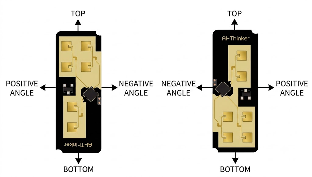
The reason is the antennas. Section one explained that this module measures direction by comparing the phase of the same echo at its two receive antennas, and that only works along the axis those two antennas are separated on. Stand the board on edge and that axis is horizontal, so the module measures left and right across the room, which is what you want. Lay it flat and the same measurement becomes up and down, so everyone in the room collapses onto the centre line of your scope and the sensor looks like it cannot see angle at all. It can; you have simply turned its field of view through ninety degrees.
Aim it into the room at roughly chest height if you can, and remember the wedge is only ±60°, so a target directly beside the board is outside it.
ORIGIN.x + t.x * SCALE and ORIGIN.y - t.y * SCALE place the blip, while the rings behind it restore the polar view the sensor started with. The practical benefit is that you can read range off the picture at a glance without doing any arithmetic, and the wedge shows you exactly where the sensor is blind. Both would be lost on a plain rectangular grid.Then press Start
Press Start in App Lab. That is the whole procedure: it builds the sketch, flashes it to the MCU, installs the Python side, brings up the Web UI Brick, and then opens your browser at the right address by itself, so there is no port to remember and no hostname to type.
If you prefer the command line, or you are already in an SSH session, the equivalent pair is:
arduino-app-cli app start ~/ArduinoApps/radar_scope
arduino-app-cli app logs  ~/ArduinoApps/radar_scope
Going this route you open the page yourself, at http://<your-board>.local:7000. Keep the logs command to hand either way, because it is the only place the Python half can tell you anything.
Now get up and walk! A green blip tracks you across the wedge, trailing its history; the readout beside it shows your range and radial speed. Bring other people in for the full three-target experience.
Video 2. The mmWave radar first run tracking me at my desk displayed live in the web page that is being generated by the Arduino UNO Q Python code.
- Make sure you are looking at the page you just edited. Before anything else, hard-reload with Ctrl-F5, and close any older tab still showing the scope. A browser tab holds its JavaScript in memory once loaded, so an old tab keeps happily running the previous version while a new one shows your edit. Having both open at once produces a baffling pair of symptoms (the same App apparently working in one window and failing in another). I lost time to precisely this.
- Read the logs next.
arduino-app-cli app logs ~/ArduinoApps/radar_scope should end with App started. and no traceback. If Python died, the Brick keeps serving the page regardless, so the browser looks fine and tells you nothing.- Then fake a target from Python, which splits the chain in half. Put this in
loop() before the sleep: ui.send_message("targets", {"targets": [{"slot": 0, "x": 0, "y": 2000, "v": 0}]})A blip 2 m dead ahead means the socket, the event name and the payload shape are all correct, and the fault is upstream.
- If the status line reads "0 target(s)" rather than "no data from the radar": messages are arriving at rate, so the connection is up and the event name matches, but the target list is coming out empty. That means the payload is not the shape the page expects. Swap the handler for a debug message.
- Then watch the Bridge. A
print("RX:", repr(raw), flush=True) at the top of on_targets shows whether the sketch is reaching Linux at all.- Finally, watch the sketch. The radar owns D0/D1, so there is no serial console to print to; use the LED instead. A
digitalWrite(LED_BUILTIN, !digitalRead(LED_BUILTIN)); where a frame passes its tail check turns "am I receiving valid frames?" into something you can see from across the room. A dark LED means the radar is not talking: check TX and RX are not swapped, and that VCC is on 5V rather than 3V3.Then run the two experiments that actually test the claims in this article.
The through-material trick. Hide the module behind a book, inside a cardboard box, or behind a wooden panel, and check that the blip does not care. This is the one party trick that impressed my teenage children, and it is the one that changes how they think about where a sensor can live.
Video 3. Two targets tracked with a sheet of cardboard between the sensor and the room. The radar does not care, which is the property no camera can match.
The still-person test, which was a genuine experiment rather than a demonstration. Sit down in front of the sensor and stop moving. I went into this expecting it to fail, for the reasons in the box back in section one, and it does not: the track holds indefinitely, and the reported speed settles at 0 cm/s. The module is telling you, in as many words, that it can see something it cannot see moving. That is breathing, and it is the capability that separates this class of sensor from every PIR ever fitted to a corridor.
Watch the position while you sit there, though, because it does something instructive. The blip does not sit perfectly still: it wanders over roughly half a metre. That is not the tracker being sloppy. Recall that 250 MHz of sweep bandwidth buys about 60 cm of range resolution, so half a metre of wander is the position estimate moving around inside a single resolution cell. The sensor is not confused about where you are; it is telling you the truth about how precisely it is able to know. You are watching ΔR = c/2B with your own eyes. The practical consequence for anything you build on this: treat a still target's position as good to about a resolution cell, and smooth it if you need better. Do not treat the wander as a fault to be engineered away, because it cannot be.
Also run the series' usual checks. Watch the scope while loading the A53 cores (yes > /dev/null four times over, as in parts 1 and 2): the page updates may stutter, but no radar frames are lost, because the parsing lives on the MCU whose loop never stopped draining the UART. And check arduino-app-cli app logs after you deliberately unplug and replug the radar's TX line: the browser should go to "no data from the radar" within a second, then recover, because the state machine resynchronises and the staleness timer reports the gap.
Part 3 of this series concluded that the matrix hardware could do 3-bit grayscale, that the mainline Zephyr driver exposed it, and that the Arduino layer did not, so the fading comet tail was a reward for going below the abstraction. That is no longer true:
setGrayscaleBits() and draw() put the same eight brightness levels in reach of an ordinary sketch. So the comet trick works here too. Decay every lit pixel by one level per frame, stamp each target at full brightness, and at roughly ten frames a second a trail lingers for about three quarters of a second, tracking a person across the panel exactly as it does across the canvas.See the Bonus Sketch attached at the end of this page.
Video 4. The final outcome of this article (and the bonus LED matrix) -- the mmWave radar sensor tracking two people in the room and displaying a web interface using only the Arduino UNO Q and the RD-03D mmWave radar.
Troubleshooting
- No frames at all. Swap TX/RX first (the eternal UART fix). Then confirm
Serial1is the D0/D1 hardware UART in your core version, and check the module is actually powered from 5V, not 3V3: an undervolted or sagging supply is a common and well-disguised cause. - Frames arrive but only ever one target. The mode-select command did not take. Either the module was still booting when it was sent (hence the
delay(200)and the repeat insetup()), or D1 is not connected: the radar will happily stream single-target frames without ever hearing from you. - Frames parse but positions are mirrored or teleport. Left/right mirroring means your mounting orientation differs from mine, so negate X. Teleporting to the far side of the scope is the sign-flag encoding being read as two's complement; reread
rd03d_decode. - Speeds have the wrong sign. The convention is asserted in the protocol table and not yet confirmed on hardware. Walk directly at the sensor and read the number; if it is negative, flip the sign in the sketch rather than in the browser, so the Bridge payload stays canonical.
- Targets flicker in and out. A motionless person should not cause this, as the still-person test above shows, so look at placement first. Deep soft furniture absorbs enough of the return to matter, an off-axis target near the ±60° edge is only weakly illuminated, and anything between you and the sensor that is not radio-transparent will attenuate. Raising the module and angling it slightly down usually helps most. If you only ever care about one person, the module's single-target mode gives a more stable track.
- Two people merge into one target. Not a bug. With 250 MHz of sweep bandwidth the range resolution is around 60 cm, and two people closer than that at the same angle are one echo. No firmware can recover them; only more bandwidth could, which the ISM allocation does not permit at 24 GHz.
- Ghost targets. Oscillating fans, monitor-stand wobble, and curtains near a heat vent are all "movers" to a Doppler radar. The demo's a fan blade preset shows what one looks like in the raw map: two bright returns at equal and opposite velocities at the same range. Aim the wedge away from them; there is no software substitute for placement.
- The scope page shows the heading and nothing else, not even the grid. That means the script never ran, so check the browser console first. A
SyntaxErrorpoints at a mangled paste;io is not definedmeanslibs/socket.io.min.jsdid not load, so check the Network tab for a 404 on it. Note the grid is drawn before the socket is touched, precisely so that a socket problem still leaves you a working page to debug from. As in Part 2, browse to the board's.localname or IP, not127.0.0.1. - The grid draws but no blips ever appear. Work through the bisection in the box under "Running it". The quickest discriminator is the status line: "no data from the radar" means nothing is arriving at all, while "0 target(s)" means messages are arriving and the target list inside them is empty.
- The scope shows a frozen blip. This should be impossible with the staleness handling in both halves, so if you see it, one of the two timers is not running: check that
loop()in the sketch is still being reached (a blocking read somewhere would stop it) and thatlastMsgis being updated in the browser. - Garbage in the MCU console, or occasional torn frames after a reset. Remember that the Zephyr console shares D0/D1 with the radar. The frame state machine is designed to shrug this off, but if a boot banner is landing in the middle of your data this is where it comes from.
Conclusion
- FMCW radar measures range from beat frequency, speed from chirp-to-chirp phase, and angle from the phase difference between two receive antennas: one elegant mechanism yielding X, Y, and velocity per target. The interactive range-Doppler demo above is the fastest way to internalise the chain, and the fastest way to see why 250 MHz of ISM bandwidth caps this module's range resolution at around 60 cm.
- That physics translates into the sensor type's practical strengths: darkness- and temperature-indifference, mounting through materials, multi-target positional tracking, image-free privacy, and, for presence-tuned parts, detection of a motionless breathing human. The zero-Doppler discussion is where that last capability is won or lost, and it is a firmware decision the module has already made for you.
- The RD-03D packages all of it behind a UART for under €10; its eccentricities (a non-standard baud rate, sign-flag integer encoding, torn-frame realities) are exactly the kind of wire-format work that belongs next to the pins, and the sketch's state machine is the reusable artefact of this post.
- The dual-brain split was relevant again, but for a different reason than the previous parts. The header UART is wired to the STM32 and to nothing else, so Linux cannot read this sensor: the division of labour was decided by the schematic. The direction of travel was new too, with the MCU initiating the Bridge call for the first time in this series, which turned out to delete a race.
The obvious next step is the one flagged in Part 2: this radar knows where things move but not what they are, and the camera knows what but works only in the light it is given. Fusing them (radar-gated inference, cross-validated presence) is where this series' two sensing threads integrate together.
Acknowledgements
My thanks to Prof. Conor Brennan of Dublin City University for reading a draft of this article and for his advice on the radar section. Any errors that remain are mine.

